How to Implement Spline Fitting

• Introduction
• Splines
• Spline Fitting - First Steps
• The Optimization Problem
• Optimizing It
• Show Me the Code!
• Challenges and Improvements
  • Avoiding Loops
  • Adding Constraints
    • Lagrange Multipliers
• Closing Words

Introduction

In this article, I’ll show you how I implemented spline fitting in Scan Tailor, which is a tool for post-processing scanned or photographed pages. I am the original author of that project and I was involved with it between 2007 and 2016.

Spline fitting is used there in the dewarping workflow (introduced around 2011), where a curved page is flattened. The picture below should give you the idea:

The better the grid follows the curvature of text lines, the better dewarping results you are going to get.

You can let Scan Tailor build the grid by itself or you can define it manually. You can also manually adjust the grid built by Scan Tailor. That’s where spline fitting comes into play. The whole grid is defined by two horizontal curves: the top and the bottom one. They don’t have to be the top-most and the bottom-most text lines, but accuracy is better when they are far apart. The other curves are automatically derived from those two. When Scan Tailor builds the grid by itself, the curves are represented by polylines. The polylines are produced by a custom image processing algorithm and look like this:

That screenshot above was taken from Scan Tailor’s debugging output (Menu -> Tools -> Debug Mode).

Now suppose the dewarping grid built for you by Scan Tailor is imperfect and you want to adjust it manually. How are you going to adjust the polylines? Certainly not point-by-point!

Splines

The standard way to manually adjust a curve is to represent that curve as a spline. A spline is a function of this form:

\[\mathbf{s}(t; \mathbf{X})\]

It takes a time / progress argument $ t $ and is parametrized by a set of control points $ \mathbf{X} $. Some types of splines may have additional parameters. For convenience we make $ \mathbf{X} $ to be a matrix whose columns are the spline’s control points. The spline function returns a vector (a 2D one in our case), which is a position on the screen.

I like to think of a spline function as of a trajectory of a particle function. It takes time and produces the position of the particle at that time. Scan Tailor uses X-splines, whose parameter $ t $ goes from 0 to 1. Those splines are parametrized by a sequence of control points and a tension parameter for each control point. On the picture below, the bottom curve is a spline with red dots being its control points. The tension parameters are not mentioned in the formula above, because we simply hardcode them. Keep reading for more details.

The red dots (barely visible) are the control points. Their positions define the shape of the spline. When Scan Tailor fits splines to polylines, it uses a fixed number of control points - 5. The user can then add more of them or remove some.

Let’s zoom in a bit:

You’ll notice the spline doesn’t actually pass through its control points. That’s because there are two types of splines - the interpolating ones (those do pass through their control points) and the approximating ones (those are merely attracted to their control points). The X-Spline is a hybrid model where the tension parameter specifies whether the spline will pass through a particular control point or merely be attracted to it, and how much. Scan Tailor doesn’t expose the tension parameters to users. It just makes the splines go through the first and the last control points and be attracted to the rest of them. Why not make the spline pass through all control points? Because then more control points would be required to represent the same curve. That’s just my empirical observation.

Spline Fitting - First Steps

So, how do we fit a spline to a polyline? It’s going to be an iterative process. We start with a spline whose first and last control points correspond to the first and the last points of the polyline and the rest of the control points are placed at equal intervals:

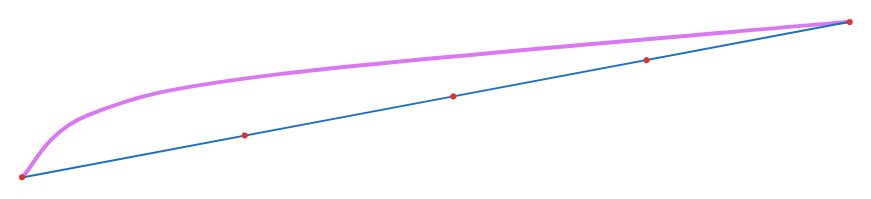
The next step is to sample the spline (place some points on the spline at more or less equal intervals) and for each such point, find the closest point to it on the polyline:

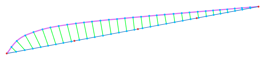
If we were fitting a spline to a point cloud rather than to a polyline (the points in a point cloud are unordered), then we would do it slightly differently: for each point in the point cloud we would find the closest point on the spline (which is a challenging problem by itself). Anyway, what we really want is a set of points on the spline with known $ t $ values and a point of attraction for each of them.

The Optimization Problem

Now we are ready to formulate our optimization problem. It’s just our initial attempt - we are going to make improvements to it later in the article. However, before I write down the formula, let me explain in simple words what it does.

We are going to find such a matrix $ \mathbf{X} $ (a collection of spline control points) that minimizes the sum of squared lengths of those green lines on the picture above. Why squared lengths? There is more than one reason, but the main one is me trying to keep the objective function quadratic, as those are easy to optimize. BTW, the term optimization in mathematics means just minimization or maximization (in this case, it’s minimization). Oh, and before I present our optimization problem in a mathematical notation, bear in mind I am a software engineer not a mathematician, so don’t judge my math too harshly but do let me know if you spot an error!

OK, here it goes:

\[f(\mathbf{X}) = \sum_{i=1}^{N}{\|\mathbf{s}(t_i, \mathbf{X}) - \mathbf{q}_i\|^2} \tag{1}\] \[\text{argmin}_{\mathbf{X}} f(\mathbf{X})\]

Where:

• $ \mathbf{X} $ is a matrix of spline’s control points.
• $ N $ is the number of samples (the green lines on the picture above).
• $ t_i $ is the spline’s parameter $ t $ for sample $ i $. It comes from the spline sampling process.
• $ \mathbf{s}(t_i, \mathbf{X}) $ is our spline function (with tension parameters treated as constants).
• $ \mathbf{q}_i $ is the attraction point for sample $ i $ (a point on the polyline closest to the given point on the spline).

OK, but $ \mathbf{s}(t; \mathbf{X}) $ is a rather complex function in case of X-splines! How do we deal with that? The thing is, it’s only complex when you treat $ t $ as a variable. In our case, $ t_i $’s are constants (and so are tension parameters) and the only real variable is $ \mathbf{X} $. Turns out, in such a setting, it reduces to:

\[\mathbf{s}(\mathbf{X}; t) = \mathbf{X}\mathbf{v}(t) \tag{2}\]

Bearing in mind that columns of $ \mathbf{X} $ are the spline’s control points, the function becomes a linear combination of those control points where $ \mathbf{v}(t) $ is a vector-valued function giving us the coefficients for that linear combination. Because $ t $ is a constant (a bunch of $ t_i $’s are produced by spline sampling we did above), we can pre-compute $ \mathbf{v}(t_i) $ for all samples.

To give you a better understanding, here is how $ \mathbf{v}(t) $ may be represented in C++ code:

class FittableSpline
{
public:
    /**
     * Computes the linear coefficients for control points for the given @p t.
     * Any extra parameters (such as tension values) a spline may have are
     * treated as constants. A linear combination of control points with
     * these coeffients produces the point on this spline at @p t.
     */
    virtual Eigen::VectorXd linearCombinationAt(double t) const = 0;

Optimizing It

With (2) being a linear function of $ \mathbf{X} $ and (1) being a quadratic function of (2), (1) must be a quadratic function of $ \mathbf{X} $. To minimize (1), we just need to compute its derivatives with respect to $ \mathbf{X} $, set them to zero and solve the resulting linear system. Easy? Not exactly. How are we going to take derivatives with respect to a matrix? They don’t teach you that in your undergraduate math courses!

What we are going to do is to bring (1) to the canonical form of a scalar-valued, multivariable quadratic function, that has well known derivatives:

\[\mathbf{x}^\top \mathbf{A} \mathbf{x} + \mathbf{b}^\top \mathbf{x} + c \tag{3}\]

Where $ \mathbf{x} $ is our matrix $ \mathbf{X} $ flattened into a vector and $ \mathbf{A} $, $ \mathbf{b} $ and $ c $ are arbitrary parameters.

Perhaps it’s worth to explain what the first term of (3) expands to:

\[\mathbf{x}^\top \mathbf{A} \mathbf{x} = \sum_{i,j}{\mathbf{x}_i \mathbf{A}_{i,j} \mathbf{x}_j}\]

Basically, we take every element of $ \mathbf{x} $, multiply it by every other element (and also the same element) and by a corresponding coefficient from matrix $ \mathbf{A} $. Then we sum up the resulting terms.

(3) has well-known gradient (the vector of first partial derivatives), which is:

\[(\mathbf{A}^\top + \mathbf{A}) \mathbf{x} + \mathbf{b} \tag{4}\]

So how exactly are we going to bring (1) into the form of (3) in order to minimize it? It turns out it’s much easier done programmatically than mathematically (for me at least). So, let’s do that in C++. If you spot an error, please tell me.

Show Me the Code!

First, we’ll need a few structs to represent various functions we’ll be dealing with.

/**
 * Represents a scalar-valued linear function of the form:
 * <pre>
 * f(x) = a^T * x + b
 * </pre>
 * where a is a vector and b is a scalar.
 */
struct ScalarLinearFunction
{
    Eigen::VectorXd a;
    double b = 0.0;

    /**
     * Sets this->a to the correct size and initializes
     * this->a and this->b with zeros.
     */
    explicit ScalarLinearFunction(size_t numVars);

    size_t numVars() const;

    ScalarLinearFunction& operator+=(ScalarLinearFunction const& other);
};

/**
 * Represents a vector-valued linear function of the form:
 * <pre>
 * f(x) = Ax + b
 * </pre>
 * where A is a matrix and b is a vector.
 */
struct VectorLinearFunction
{
    Eigen::MatrixXd A;
    Eigen::VectorXd b;
};

/**
 * Represents a scalar-valued quadratic function of the form:
 * <pre>
 * f(x) = x^T * A * x + b^T * x + c
 * </pre>
 * where A is a matrix, b is a vector and c is a scalar.
 */
struct ScalarQuadraticFunction
{
    Eigen::MatrixXd A;
    Eigen::VectorXd b;
    double c = 0.0;

    /**
     * Sets this->A and this->b to the correct sizes and initializes
     * this->A, this->b and this->c with zeros.
     */
    explicit QuadraticFunction(size_t numVars);

    size_t numVars() const;

    VectorLinearFunction gradient() const;

    ScalarQuadraticFunction& operator+=(ScalarQuadraticFunction const& other);
};

ScalarLinearFunction operator+(
    ScalarLinearFunction const& lhs, ScalarLinearFunction const& rhs);

ScalarQuadraticFunction operator+(
    ScalarQuadraticFunction const& lhs, ScalarQuadraticFunction const& rhs);

ScalarQuadraticFunction operator*(
    ScalarLinearFunction const& lhs, ScalarLinearFunction const& rhs);

Apart from the gradient computation (4), the only other non-trivial operation above is the multiplication of two ScalarLinearFunction’s to produce a ScalarQuadraticFunction. It can be implemented using the following relationship:

\[(\mathbf{a}_1^\top \mathbf{x} + b_1)(\mathbf{a}_2^\top \mathbf{x} + b_2) = \mathbf{x}^\top (\mathbf{a}_1 \mathbf{a}_2^\top) \mathbf{x} + (\mathbf{a}_1 b_2 + \mathbf{a}_2 b_1)^\top \mathbf{x} + b_1 b_2\]

Assuming we’ve implemented all the methods mentioned above, we can now transform (1) to (3):

struct SplineSample
{
    /**
     * Spline parameter t.
     */
    double t;

    /**
     * The point on the polyline to which spline(t) shall be attracted.
     */
    Eigen:Vector2d attractionPoint;
};

ScalarQuadraticFunction buildObjectiveFunction(
    FittableSpline const& spline, std::vector<SplineSample> const& samples)
{
    size_t const numControlPoints = spline.numControlPoints();

    // Each control point carries 2 variables: its x and y coordinates.
    size_t const numVars = numControlPoints * 2;

    // Initialized with zeros.
    ScalarQuadraticFunction objectiveFunction(numVars);

    for (SplineSample const& sample : samples)
    {
        Eigen::VectorXd const controlPointWeights =
            spline.linearCombinationAt(sample.t);

        // We use two separate linear functions to represent the horizontal
        // and vertical components of `s(t_i, X) - q_i`.
        ScalarLinearFunction deltaX(numVars);  // Initialized with zeros.
        ScalarLinearFunction deltaY(numVars);  // Initialized with zeros.

        deltaX.b = -sample.attractionPoint(0);
        deltaY.b = -sample.attractionPoint(1);

        for (size_t i = 0; i < numVars; ++i)
        {
            // Even indices of vector x correspond to the x coordinates
            // of control points.
            deltaX.a(i * 2) = controlPointWeights(i);

            // Odd indices of vector x correspond to the y coordinates
            // of control points.
            deltaY.a(i * 2 + 1) = controlPointWeights(i);
        }

        objectiveFunction += deltaX * deltaX + deltaY * deltaY;
    }

    return objectiveFunction;
}

Now, to solve for $ \mathbf{x} $ (the flattened collection of spline control points), we just have to set the gradient to zero and solve the resulting linear system:

ScalarQuadraticFunction const objectiveFunction =
    buildObjectiveFunction(spline, samplesOfSpline);

VectorLinearFunction const gradient = objectiveFunction.gradient();

auto qr = gradient.A.colPivHouseholderQr();
if (!qr.isInvertible())
{
    // Handle error.
}

Eigen::VectorXd const x = qr.solve(-gradient.b);

That gives us the new positions of spline’s control points that minimize the sum of squared lengths of those green lines on the picture. Then, we repeat the whole process starting from spline sampling, and keep repeating it until the average squared length of a green line stops reducing.

Challenges and Improvements

Unfortunately, the approach described above doesn’t work that well. You may well end up with a result like this:

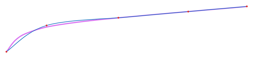
The root cause of such a poor fit is that our objective function (1) discourages the lateral movement of spline control points, as such a movement would lead to the average length of a green line increasing.

Basically, this:

would become this:

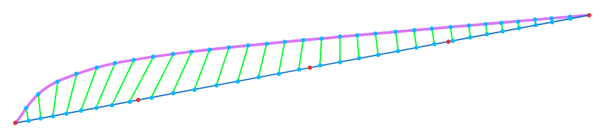
As can be seen, the green lines would longer which is something our objective function really fights against!

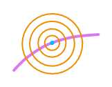
And yet, we do need more control points where the polyline curves more, in order to represent that curvature. What can we do about it? Well, we could improve the initial positioning of control points, so that more control points are placed in high curvature zones. However, that alone would probably not be enough. A better way is to change our objective function. Our initial objective function (1) penalizes displacements relative to the attraction point equally in all directions. See the isocontours of that penalty function:

What we need is a penalty function what penalizes the displacements along the spline less than those in the orthogonal direction:

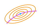
Each ellipse represents a constant level of penalty. So, on the same penalty budget we can now afford a larger displacement along the polyline than in the orthogonal direction.

How much do we stretch those isocontours? We stretch them more in low curvature areas and less in high curvature ones. This article is getting longer than I would like it to be, so I am not giving the full details here, but you can find them in these two papers (1, 2). Also take a look at the relevant code in Scan Tailor. What’s important is that the modified objective function is still quadratic, so we optimize it exactly the same way.

Does the above help? It does, but it solves one problem and creates two more:

1. When trying to fit a spline to a more or less flat polyline, loops are occasionally created:
2. The spline endpoints may end up far from the polyline endpoints.

Let’s solve each of the above problems.

Avoiding Loops

The 1st problem is solved by adding another penalty term to (1) that penalizes the sum of squared distances between the adjacent control points, or alternatively, between points on the spline corresponding to adjacent control points. The 1st option is going look like this:

\[\alpha \sum_{i=1}^{K-1}{\|\mathbf{X}_{i+1} - \mathbf{X}_i\|^2}\]

Where:

• $ \alpha $ is the importance factor of this penalty term. We start with a higher value and gradually reduce it in subsequent iterations.
• $ K $ is the number of control points in a spline.
• $ \mathbf{X}_i $ is the $ i $’th column of matrix $ \mathbf{X} $, that is the $ i $’th control point of the spline.

Adding Constraints

The 2nd problem is solved by adding constraints to our optimization problem. We need two such constraints: $ \mathbf{X}\mathbf{v}(0) = \mathbf{q}_{first} $ and $ \mathbf{X}\mathbf{v}(1) = \mathbf{q}_{last} $.

Where:

• $ \mathbf{v}(0) $ and $ \mathbf{v}(1) $ are the coefficients of linear combinations of spline’s control points that produce the start and the end point of the spline respectively.
• $ \mathbf{q}_{first} $ and $ \mathbf{q}_{last} $ are the first and the last points of the target polyline respectively.

Lagrange Multipliers

Whenever you hear about optimization under equality constraints, Lagrange Multipliers should come to mind. In fact, this is the perfect use case for them: a quadratic objective function with linear equality constraints is as easy to optimize as a quadratic function without constraints - the linear system just gets a bit larger.

Let me remind you how to use the method of Lagrange multipliers to add constraints to an optimization problem. Suppose, you need to optimize (maximize or minimize) a general, scalar-valued function $ g(\mathbf{x}) $ (where $ \mathbf{x} $ is a vector) subject to $ M $ constraints of the form $ h_i(\mathbf{x}) = c_i $ (where $ c_i $ are constants). The solution is to solve the following system of equations for $ \mathbf{x} $ and $ \mathbf{\lambda} $:

\[\begin{align} \nabla g(\mathbf{x}) &= \sum_{i=1}^M{\mathbf{\lambda}_i \nabla h_i(\mathbf{x})} \notag \\ h_1(\mathbf{x}) &= c_1 \notag \\ \vdots \notag \\ h_M(\mathbf{x}) &= c_M \notag \\ \end{align}\]

In plain English: you solve for the constraints with an additional condition that the gradient of the objective function is a linear combination of gradients of constraints. The coeffiecints ($ \mathbf{\lambda}_i $) in that linear combination are called Lagrange multipliers.

Closing Words

That’s it more or less. I had to skip some details in order to keep the article’s length reasonable, but if you still remember some Linear Algebra and some Calculus, it should be quite possible for you to fill those gaps and implement spline fitting for your project. For reference, check out Scan Tailor’s implementation.

BTW, the author may be available for contracting work.